Monte Carlo Simulation with Python and Fantasy Football
In this notebook, we’ll apply simulation (aka Monte Carlo analysis) to fantasy football. Hopefully this gives you a sense of how simulation techniques are used and why they’re so powerful.
Don’t hestate to reach out with any feedback or questions, I’m on twitter/x at @nathanbraun and my email is nate@nathanbraun.com.
How to think about fantasy football
-
Every week, a player’s fantasy score is a random draw from some distribution.
-
The shape of this distribution is different for every player, every week.
What factors go into it? Anything that might affect performance (talent, opportunity, quality of the opposing defense, how good the player’s offensive line is, weather, etc).
-
Your job as a fantasy football player is to assemble a lineup of guys with distributions as far to the right as you can. This is what maximizes your probability of winning.
Make sense? If you’re skeptical or that’s unclear check out the appendix at the end of this notebook. We build up the intuition behind it there.
Working with fantasy distributions
So we want to maximize our probability of winning by picking the guys with the best distributions. How might we do that?
Option 1 for working with distributions: math
The first way to work with distributions is by manipulating certain mathematical equations that — when plotted with X, Y coordinates — make curves.
For example, given some numbers for average and standard deviation , you could draw a Normal distribution by plotting this equation:
But there are some issues:
- One is that it restricts you to certain types of curves and shapes. This equation is for a Normal distribution. Other equations have other names. Gamma, Poisson, Weibull, etc. There are a lot of curves, but even so, not all data follows these shapes.
- An even bigger bigger problem is that working with the math involved is tedious and difficult at best and literally impossible at worse.
Say I told you Justin Herbert and Patrick Mahomes’s projections this week are both normally distributed ~N(18,6) and ~N(20.5,7) respectively.
Quick, using the equation above, tell me — what’s the probability Justin Herbert scores more than Patrick Mahomes? Hopefully you paid attention in calculus.
Option 2 for working with distributions: simulations
Simulations are a much easier way of working with distributions. Analysis that works with simulations is also called Monte Carlo analysis.
Technically, simulations are a bunch of draws from some data generating process. Often that process is a mathematical distribution like a Normal or Gamma distribution. But we can also work with data generating processes that are difficult or impossible to describe mathematically. In that case simulations are our only option.
In practice, most simulation analysis involves:
- Generating data according to some process that reflects the aspects of reality you care about. Sometimes this means finding the right distribution, other times it means combining distributions or generating data according to other rules.
- Asking questions and analyzing this simulated data via summary statistics or plots.
Here, I’ve taken care of (1) for you by modeling thousands of simulated fantasy scores for each player. In this notebook, we’ll go through some cool examples of (2) using this simulation data to ask different questions.
A note on this document
This is a Jupyter notebook, which is a way to show a mixture of text, tables and Python code.
You don’t have to worry about the code (the parts with In [ ] next to them) if you don’t want. What’s important is the code’s output (the parts next to Out[ ]), which are usually interesting numbers, data tables or graphs that I’ll reference in the text.
Note if you are interested in the code (awesome!) you can still read through the document as is, and I’d recommend starting there. Eventually if you want play around with this yourself and change any of the code you have two options:
-
If you have some basic familiarity with Python, Jupyter and Github, you can clone the repository and run it on your local machine. Or
-
You can run the notebook in binder (a free, interactive Jupyter notebook viewer) by clicking on the following link:
https://mybinder.org/v2/gh/nathanbraun/fantasy-monte-carlo/main?filepath=fantasy-monte-carlo.ipynb
Note binder is creating a mini computer environment takes a few minutes to get set up.
Monte Carlo Analysis for Week 3, 2023
Loading the data
Let’s look at some player simulations from Week 3, 2023.
import pandas as pd
pd.options.mode.chained_assignment = None

nsims = pd.read_csv('./data/nsims.csv')
nsims| patrick-mahomes | jalen-hurts | josh-allen | joshua-dobbs | zach-wilson | lamar-jackson | justin-herbert | tua-tagovailoa | trevor-lawrence | kirk-cousins | ... | no | tb | jax | was | den | det | pit | sf | atl | lv | |
|---|---|---|---|---|---|---|---|---|---|---|---|---|---|---|---|---|---|---|---|---|---|
| 0 | 31.373173 | 22.943242 | 31.278690 | 5.930377 | 28.441495 | 14.373618 | 24.889975 | 15.949190 | 21.141992 | 36.369677 | ... | 12.254481 | 1.352437 | 11.359663 | 3.107871 | 3.792302 | 8.339201 | 13.518176 | 11.165673 | 16.655954 | 0.079218 |
| 1 | 15.580346 | 21.278506 | 18.328942 | 19.028315 | 8.589043 | 24.928424 | 19.695595 | 27.723994 | 7.001144 | 20.165356 | ... | 9.880197 | 7.885957 | 5.417069 | 6.630614 | 0.234699 | 14.633196 | 14.348552 | 13.227680 | 14.725048 | 7.598453 |
| 2 | 19.305332 | 20.131436 | 26.930733 | 12.247553 | 10.167820 | 21.200463 | 25.814006 | 23.920744 | 14.738819 | 30.615639 | ... | 9.225533 | 3.289643 | 27.502175 | 1.235033 | 14.118362 | 6.083915 | 1.695059 | 0.826584 | 0.677490 | 11.846076 |
| 3 | 5.358195 | 32.302340 | 24.790600 | 9.920325 | 12.176310 | 14.476399 | 14.212815 | 21.219843 | 25.647645 | 12.746029 | ... | 8.700703 | 6.431883 | 3.332168 | 6.274708 | 4.677788 | 5.958758 | 2.251701 | 15.044705 | 15.128840 | 9.830206 |
| 4 | 19.384985 | 39.341403 | 21.696812 | 0.924227 | 17.978923 | 22.401451 | 22.572415 | 27.873269 | 19.385690 | 9.148723 | ... | 0.969503 | 0.879348 | 1.998910 | 3.879241 | 2.155402 | 1.202186 | 5.606427 | 2.144904 | 12.699372 | 13.258936 |
| ... | ... | ... | ... | ... | ... | ... | ... | ... | ... | ... | ... | ... | ... | ... | ... | ... | ... | ... | ... | ... | ... |
| 495 | 29.309151 | 8.610684 | 25.650817 | 25.681485 | 15.598120 | 23.251073 | 18.466861 | 30.887997 | 9.937433 | 28.256653 | ... | 7.856577 | 8.067598 | 12.974184 | 9.499197 | 1.688407 | 12.076029 | 9.860445 | 10.466341 | 8.506554 | 0.583851 |
| 496 | 22.003163 | 12.419327 | 19.515395 | 5.165373 | 3.792943 | 25.437858 | 24.468821 | 30.496252 | 19.506345 | 15.723808 | ... | 13.065573 | 4.228264 | 21.554995 | 2.240510 | 0.835478 | 7.838885 | 0.051396 | 21.270722 | 6.544969 | 33.984122 |
| 497 | 36.987431 | 33.933994 | 9.371574 | 13.204348 | 8.259211 | 17.447672 | 29.982914 | 30.707705 | 11.213160 | 33.280860 | ... | 9.763586 | 0.066865 | 12.461045 | 19.515229 | 0.805873 | 29.486924 | 18.315689 | 7.870380 | 12.991355 | 10.551414 |
| 498 | 36.255033 | 27.546682 | 21.582154 | 5.769464 | 6.548873 | 25.852185 | 18.005356 | 19.560092 | 21.850911 | 16.285168 | ... | 0.272662 | 1.120690 | 18.483037 | 1.635620 | 4.197196 | 1.376383 | 0.430669 | 0.428591 | 4.276003 | 16.353748 |
| 499 | 19.389948 | 7.167897 | 15.029804 | 1.312190 | 0.808112 | 1.428399 | 21.476163 | 25.916025 | 27.177536 | 27.330606 | ... | 9.510551 | 2.594103 | 3.499939 | 5.174932 | 1.263133 | 3.921430 | 7.067016 | 9.664141 | 4.373769 | 16.553160 |
500 rows × 283 columns
This is our simulation data. Each column holds draws from a players distribution, which are numbered (on the side) 0, 1, … 499. In theory, we could draw as many simulations as we want. To keep things loading fast I’ve limited each player to 500 simulations.
More info on the players we’re simulating — including position, team, and the number of points they actually ended up scoring in week 3, 2023 is here:
players = (pd.read_csv('./data/players.csv')
           .assign(player_id=lambda df: df['player_id'].astype(str))
           .set_index('player_id'))
players.head()| name | pos | team | actual | |
|---|---|---|---|---|
| player_id | ||||
| 1091 | Patrick Mahomes | QB | KC | 25.68 |
| 498 | Jalen Hurts | QB | PHI | 19.88 |
| 889 | Josh Allen | QB | BUF | 21.32 |
| 1094 | Joshua Dobbs | QB | ARI | 17.06 |
| 329 | Zach Wilson | QB | NYJ | 6.38 |
Descriptive statistics
So it’s week 3, 2023 and we have our data.
Let’s take a player, say Justin Herbert. 500 simulations. What can we do with this?
Well, if we’re interested in projecting how many points he’ll score we could take the average value of our simulations:
print(nsims['justin-herbert'].mean())21.976058849476672
Or we can look at the median:
print(nsims['justin-herbert'].median())21.55108079040353
But the real benefit of simulations is how they let you work with distributions. We can get a sense of the distribution with summary statistics:
print(nsims['justin-herbert'].describe(percentiles=[0.05, .25, .5, .75, .95]))count 500.000000 mean 21.976059 std 8.513235 min 0.606958 5% 9.045559 25% 15.900111 50% 21.551081 75% 27.480257 95% 36.132164 max 49.746482 Name: justin-herbert, dtype: float64
Or by visualizing it:
import seaborn as sns
g = sns.FacetGrid(nsims, aspect=2)
g = g.map(sns.kdeplot, 'justin-herbert', fill=True)
g.fig.subplots_adjust(top=0.9)
g.fig.suptitle("Justin Herbert's Fantasy Points Distribution - Wk 3, 2023")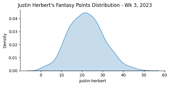
Will Herbert outscore Mahomes?
Remember above, when I asked for the probability Justin Herbert outscores Mahomes?
With our data, figuring this out is easy. We have:
nsims[['justin-herbert', 'patrick-mahomes']]| justin-herbert | patrick-mahomes | |
|---|---|---|
| 0 | 24.889975 | 31.373173 |
| 1 | 19.695595 | 15.580346 |
| 2 | 25.814006 | 19.305332 |
| 3 | 14.212815 | 5.358195 |
| 4 | 22.572415 | 19.384985 |
| ... | ... | ... |
| 495 | 18.466861 | 29.309151 |
| 496 | 24.468821 | 22.003163 |
| 497 | 29.982914 | 36.987431 |
| 498 | 18.005356 | 36.255033 |
| 499 | 21.476163 | 19.389948 |
500 rows × 2 columns
Then it’s just a matter of — did Herbert outscore Mahomes in our simulations? True or False:
(nsims['justin-herbert'] > nsims['patrick-mahomes'])0 False
1 True
2 True
3 True
4 True
...
495 False
496 True
497 False
498 False
499 True
Length: 500, dtype: bool
And taking the average (True is 1, False is 0):
print((nsims['justin-herbert'] > nsims['patrick-mahomes']).mean())0.426
So Herbert is projected to outscore Mahomes 42.6% of the time.
This means Mahomes distribution is further to the right. If we want to see what that looks like:
nsims_long = nsims[['justin-herbert', 'patrick-mahomes']].stack().reset_index()
nsims_long.columns = ['sim_n', 'player', 'pts']

g = sns.FacetGrid(nsims_long, hue='player', aspect=2)
g.map(sns.kdeplot, 'pts', fill=True)
g.add_legend()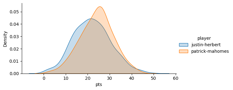
Other Monte Carlo Applications
What else can we ask?
When working with simulations, you’re really only limited by your imagination. For example, what’s the probability Justin Herbert outscores both Matt Stafford AND Justin Fields by at least 11.5 points?
Can you imagine working with the probability distribution equations above to figure that out mathematically? But, again, with our nsims data it’s easy:
print((nsims['justin-herbert'] >
         nsims[['matthew-stafford', 'justin-fields']].max(axis=1) + 11.5).mean())
0.158
So about a 16% chance Herbert outscores both Stafford and Fields by at least 11.5 points.
The other benefit: Monte Carlo analysis is flexible. You can take into account whatever you want, as long as you figure out how to build it into the data generating process.
Projecting best ball distributions
For example, say we’re interested in projecting QB points for our best ball team, where we have both Herbert and Matthew Stafford.
This is something that’s impossible to figure out numerically, but easy to build into your simulation:
- Take a draw from each player, then —
- Use the higher of the two scores for your QB spot .
- Analyze that QB score with some basic summary stats.
In this case our data generating process isn’t just approximating reality, it’s describing it exactly. This is how best ball leagues work.
nsims['bb_qb'] = nsims[['justin-herbert', 'matthew-stafford']].max(axis=1)

nsims[['bb_qb', 'justin-herbert', 'matthew-stafford']].describe()| bb_qb | justin-herbert | matthew-stafford | |
|---|---|---|---|
| count | 500.000000 | 500.000000 | 500.000000 |
| mean | 24.183287 | 21.976059 | 15.842432 |
| std | 7.519747 | 8.513235 | 8.145466 |
| min | 4.254415 | 0.606958 | 0.027773 |
| 25% | 19.197732 | 15.900111 | 9.984359 |
| 50% | 23.801324 | 21.551081 | 15.836984 |
| 75% | 28.720037 | 27.480257 | 21.395072 |
| max | 49.746482 | 49.746482 | 40.711039 |
So on average, we’d expect a best ball duo of Herbert and Stafford to score about 24.18 points, vs 21.98 and 15.84 for Herbert and Stafford individually.
What if we want to see how much adding Kirk Cousins would raise our score?
nsims['bb_qb2'] = nsims[['justin-herbert', 'matthew-stafford', 'kirk-cousins']].max(axis=1)

nsims[['bb_qb2', 'bb_qb', 'justin-herbert', 'matthew-stafford', 'kirk-cousins']].describe().round(2)| bb_qb2 | bb_qb | justin-herbert | matthew-stafford | kirk-cousins | |
|---|---|---|---|---|---|
| count | 500.00 | 500.00 | 500.00 | 500.00 | 500.00 |
| mean | 27.03 | 24.18 | 21.98 | 15.84 | 21.64 |
| std | 7.01 | 7.52 | 8.51 | 8.15 | 8.15 |
| min | 12.35 | 4.25 | 0.61 | 0.03 | 0.37 |
| 25% | 22.15 | 19.20 | 15.90 | 9.98 | 16.07 |
| 50% | 26.38 | 23.80 | 21.55 | 15.84 | 20.99 |
| 75% | 31.69 | 28.72 | 27.48 | 21.40 | 26.96 |
| max | 52.09 | 49.75 | 49.75 | 40.71 | 52.09 |
That brings the average up 3 points, to 27.
By modifying the data generating process and drawing a bunch of simulations, we’re able to answer questions about our data it’d be impossible to figure out any other way.
It’s also interesting to plot these distributions:
nsims_long = nsims[['justin-herbert', 'matthew-stafford', 'kirk-cousins', 'bb_qb', 'bb_qb2']].stack().reset_index()
nsims_long.columns = ['sim_n', 'player', 'pts']

g = sns.FacetGrid(nsims_long, hue='player', aspect=2)
g.map(sns.kdeplot, 'pts', fill=True)
g.add_legend()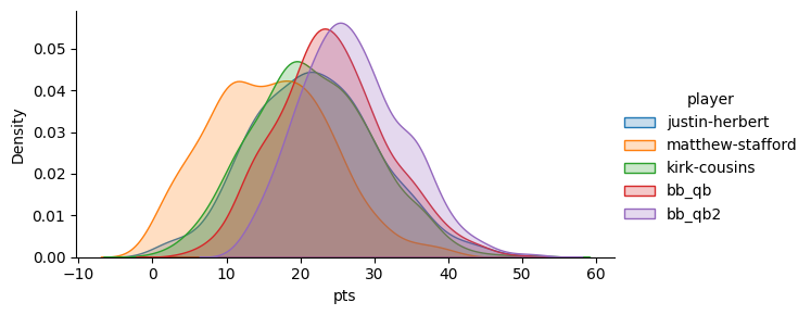
Interlude - how are these simulations calculated anyway?
Good question. For the very first version of these simulations I figured out a good Gamma distribution for each player, and took draws from that.
A Gamma distribution is shaped similarly to a Normal distribution, but more skewed. Just like a normal distribution has parameters and for average and standard deviation, a gamma distribution has parameters named and . The formula for it is:
where is:
So the first version of these simulations involved (a) figuring out the best gamma distribution (i.e. the best values of and ) for each player, and (b) taking a bunch of random draws (the simulations) from that.
These formulas look intimidating, but in practice this is mostly done with code. You tell the computer to figure out the best values of and to match real world data. The factors that went into it:
- weekly expert consensus rankings (higher ranked players are better, players who experts are split on have wider ranges of outcomes)
- betting info, i.e. team totals, opponent totals, and spreads.
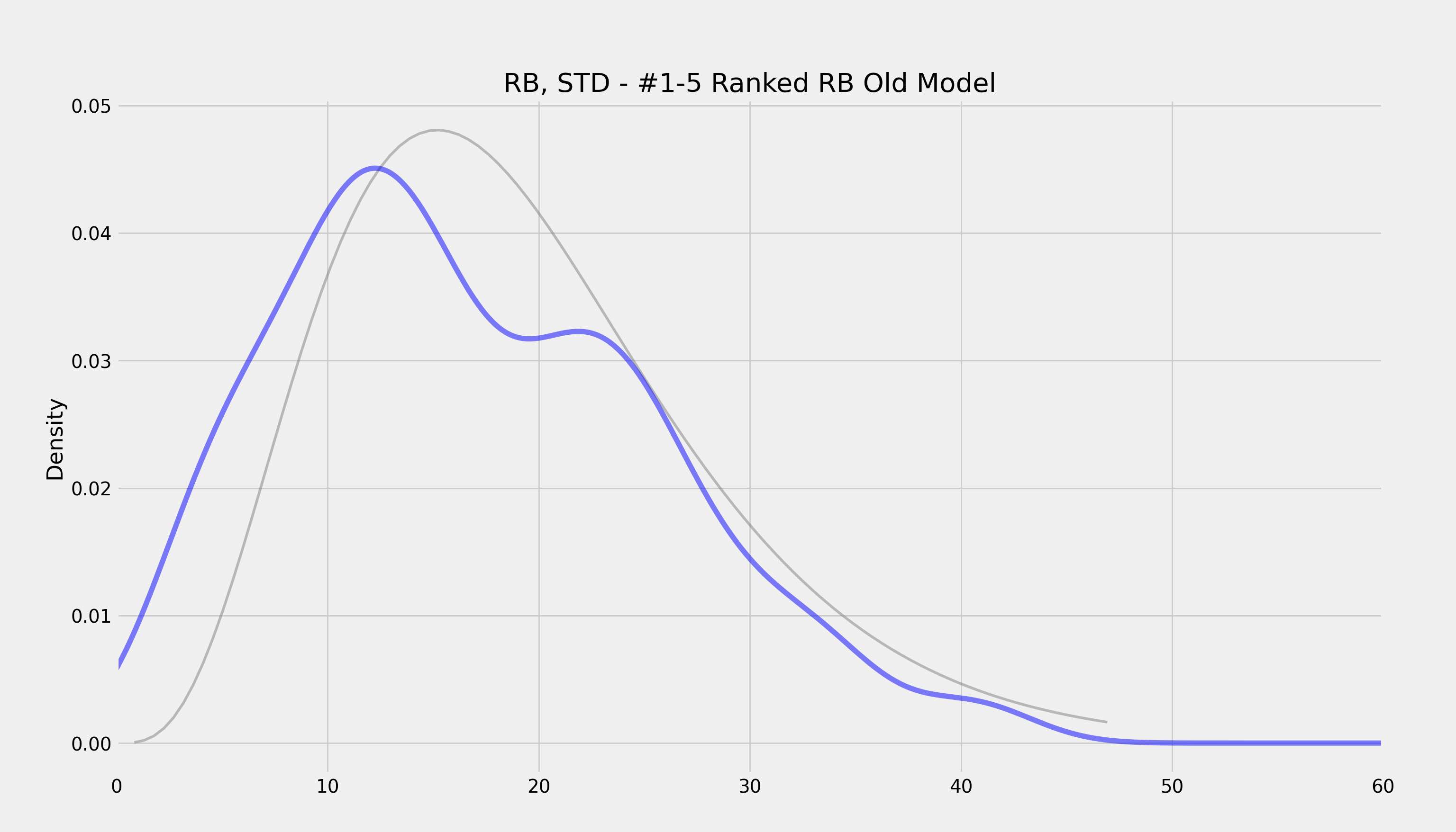
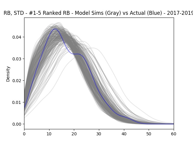
That was the first version of these simulations. Since then I’ve switched to a fancier modeling technique that basically blends a bunch of distributions together. So rather than one gamma curve, it’s a bunch of curves. This lets the model be much more flexible.
The two models (gray curves) and how they compare with the distribution of actual points scored (blue curve) are here:
Actual scores vs projections
Because we’re looking at data from last year, we know how many points these players actually scored, it’s the actual column of our player data:
players| name | pos | team | actual | |
|---|---|---|---|---|
| player_id | ||||
| 1091 | Patrick Mahomes | QB | KC | 25.68 |
| 498 | Jalen Hurts | QB | PHI | 19.88 |
| 889 | Josh Allen | QB | BUF | 21.32 |
| 1094 | Joshua Dobbs | QB | ARI | 17.06 |
| 329 | Zach Wilson | QB | NYJ | 6.38 |
| ... | ... | ... | ... | ... |
| 5161 | DET | DST | DET | 16.00 |
| 5177 | PIT | DST | PIT | 14.00 |
| 5179 | SF | DST | SF | 8.00 |
| 5152 | ATL | DST | ATL | 3.00 |
| 5169 | LV | DST | LV | 2.00 |
283 rows × 4 columns
So Mahomes scored 25.68 points in Week 2, 2023. How does that compare with what we simulated for him beforehand?
Well, our median Mahomes simulation was:
print(nsims['patrick-mahomes'].median())24.493723591765647
So it’s pretty close.
What about percentile-wise?
print((25.68 > nsims['patrick-mahomes']).mean())0.56
So Mahomes score in Week 3 beat 56% of his simulations, i.e. it was a 56th percentile score.
Let’s get projected score — by taking the average of the simulations — for all the quarterbacks.
(Note to do that I’m loading in another copy of our simulation data sims that’s exactly the same as nsims, but with player_id as the column titles instead of first-last name.)
sims = pd.read_csv('./data/sims.csv')

qbs = players.loc[players['pos'] == 'QB']
qbs['proj'] = sims.mean().round(2)

qbs.sort_values('proj', ascending=False).head(15)[['name', 'proj', 'actual']]| name | proj | actual | |
|---|---|---|---|
| player_id | |||
| 1091 | Patrick Mahomes | 24.11 | 25.68 |
| 494 | Justin Herbert | 21.98 | 29.30 |
| 2085 | Kirk Cousins | 21.64 | 25.68 |
| 498 | Jalen Hurts | 21.35 | 19.88 |
| 893 | Lamar Jackson | 21.24 | 28.18 |
| 889 | Josh Allen | 21.01 | 21.32 |
| 493 | Tua Tagovailoa | 19.95 | 28.36 |
| 327 | Trevor Lawrence | 19.10 | 14.36 |
| 1297 | Dak Prescott | 18.67 | 14.36 |
| 1883 | Geno Smith | 17.72 | 15.44 |
| 328 | Justin Fields | 17.56 | 10.66 |
| 1088 | Deshaun Watson | 17.25 | 21.16 |
| 492 | Joe Burrow | 17.24 | 8.16 |
| 1288 | Jared Goff | 17.19 | 18.02 |
| 156 | Brock Purdy | 16.61 | 20.30 |
Now let’s calculate each quarterback’s percentile too:
def fpts_pctile(row):
    return (row['actual'] > sims[str(row.name)]).mean()

qbs['pctile'] = qbs.apply(fpts_pctile, axis=1)
Here are the top 15 projected QBs and how they did:
qbs.sort_values('proj', ascending=False).head(15)[['name', 'proj', 'actual', 'pctile']]| name | proj | actual | pctile | |
|---|---|---|---|---|
| player_id | ||||
| 1091 | Patrick Mahomes | 24.11 | 25.68 | 0.560 |
| 494 | Justin Herbert | 21.98 | 29.30 | 0.808 |
| 2085 | Kirk Cousins | 21.64 | 25.68 | 0.694 |
| 498 | Jalen Hurts | 21.35 | 19.88 | 0.394 |
| 893 | Lamar Jackson | 21.24 | 28.18 | 0.808 |
| 889 | Josh Allen | 21.01 | 21.32 | 0.536 |
| 493 | Tua Tagovailoa | 19.95 | 28.36 | 0.854 |
| 327 | Trevor Lawrence | 19.10 | 14.36 | 0.246 |
| 1297 | Dak Prescott | 18.67 | 14.36 | 0.284 |
| 1883 | Geno Smith | 17.72 | 15.44 | 0.402 |
| 328 | Justin Fields | 17.56 | 10.66 | 0.206 |
| 1088 | Deshaun Watson | 17.25 | 21.16 | 0.706 |
| 492 | Joe Burrow | 17.24 | 8.16 | 0.136 |
| 1288 | Jared Goff | 17.19 | 18.02 | 0.558 |
| 156 | Brock Purdy | 16.61 | 20.30 | 0.688 |
So Justin Herbert scored 29.30 points vs his projection of 21.98. About an 80th percentile week. We’d expect to see an 80th performance about 1 out of every 5 times. And sure enough, if you look at the 15 players above, three of them (Herbert, Lamar Jackson, Deshaun Watson) have a pctile > 80.
Similarly, we should expect to see 10% of the players under 10 pctile, 20% under 20, etc. And actually it’s pretty close:
qbs['pctile'].describe(percentiles=[.1, .2, .3, .4, .5, .6, .7, .8, .9]).round(2)count 31.00 mean 0.49 std 0.26 min 0.01 10% 0.14 20% 0.23 30% 0.29 40% 0.39 50% 0.52 60% 0.56 70% 0.69 80% 0.74 90% 0.81 max 0.89 Name: pctile, dtype: float64
14% of players had 10th percentile or less draws, 23% of players, 20th percentile, etc.
This is the sign of a good model.
Percentiles as luck
A player’s actual point percentile is one way to quantify “luck”.
Good draws from further right in the distrubution have higher percentiles, and are luckier. Worse draws, from further left, are unlucky.
Let’s look at the top 10 luckiest fantasy QB performances in Week 3, 2023:
qbs.sort_values('pctile', ascending=False).head(10)[['name', 'proj', 'actual', 'pctile']]| name | proj | actual | pctile | |
|---|---|---|---|---|
| player_id | ||||
| 497 | Jordan Love | 14.49 | 24.26 | 0.892 |
| 2301 | Andy Dalton | 12.94 | 23.54 | 0.884 |
| 493 | Tua Tagovailoa | 19.95 | 28.36 | 0.854 |
| 1094 | Joshua Dobbs | 11.12 | 17.06 | 0.808 |
| 893 | Lamar Jackson | 21.24 | 28.18 | 0.808 |
| 494 | Justin Herbert | 21.98 | 29.30 | 0.808 |
| 150 | Kenny Pickett | 13.83 | 18.50 | 0.738 |
| 1757 | Jimmy Garoppolo | 13.19 | 17.66 | 0.716 |
| 1088 | Deshaun Watson | 17.25 | 21.16 | 0.706 |
| 2085 | Kirk Cousins | 21.64 | 25.68 | 0.694 |
(Aside: remember — this is from week 3, 2023. Now in 2024, we know Jordan Love is good (he just became the highest paid QB ever). But these distributions were built using the best information we had in September 2023. Back then opinions about Love were much more up in the air, which meant his projected distribution was further to the left. So while Love might have been good the whole time, and his success isn’t “luck” from his POV, you were indeed lucky (or ahead of the fantasy consensus) to get these kind of points out of Love back in early 2023.)
And here are the unluckiest players:
qbs.sort_values('pctile', ascending=True).head(10)[['name', 'proj', 'actual', 'pctile']]| name | proj | actual | pctile | |
|---|---|---|---|---|
| player_id | ||||
| 151 | Sam Howell | 13.30 | 0.60 | 0.014 |
| 677 | Daniel Jones | 14.63 | 3.98 | 0.082 |
| 492 | Joe Burrow | 17.24 | 8.16 | 0.136 |
| 2082 | Ryan Tannehill | 11.63 | 4.16 | 0.140 |
| 328 | Justin Fields | 17.56 | 10.66 | 0.206 |
| 155 | Desmond Ridder | 12.83 | 6.34 | 0.216 |
| 1689 | Derek Carr | 14.40 | 8.12 | 0.232 |
| 327 | Trevor Lawrence | 19.10 | 14.36 | 0.246 |
| 1297 | Dak Prescott | 18.67 | 14.36 | 0.284 |
| 890 | Baker Mayfield | 14.47 | 10.04 | 0.290 |
(Note you could reverse what we Love above and apply it to someone like Fields or Lawrence)
Would you rather be lucky or good?
Would you rather be lucky or good? Well it depends.
Patrick Mahomes is good. He has a very rightward projected point distribution.
He wasn’t particularly lucky in week 3, with a 56th percentile draw.
But because he’s good, that still meant 25.68 points. Meanwhile, Andy Dalton was very lucky in week 3 (88th percentile draw), but since he’s not that good (the median of his distribution is about 13 points) he still scored less than Mahomes.
So really, the best performing players are usually lucky and good. We can see that by looking at the top performers:
qbs.sort_values('actual', ascending=False).head(10)[['name', 'proj', 'actual', 'pctile']]| name | proj | actual | pctile | |
|---|---|---|---|---|
| player_id | ||||
| 494 | Justin Herbert | 21.98 | 29.30 | 0.808 |
| 493 | Tua Tagovailoa | 19.95 | 28.36 | 0.854 |
| 893 | Lamar Jackson | 21.24 | 28.18 | 0.808 |
| 1091 | Patrick Mahomes | 24.11 | 25.68 | 0.560 |
| 2085 | Kirk Cousins | 21.64 | 25.68 | 0.694 |
| 497 | Jordan Love | 14.49 | 24.26 | 0.892 |
| 2301 | Andy Dalton | 12.94 | 23.54 | 0.884 |
| 889 | Josh Allen | 21.01 | 21.32 | 0.536 |
| 1088 | Deshaun Watson | 17.25 | 21.16 | 0.706 |
| 156 | Brock Purdy | 16.61 | 20.30 | 0.688 |
Two of the top three are good QBs (Herbert and Lamar) who got fairly lucky (80th percentile) draws. There’s also Tua, who is a bit less good but got an even luckier draw (85th percentile). Then there’s Mahomes.
In reality, high score are a combo of luck and skill. But, since you can’t predict luck, you should just focus on the skill part, which is what you do when you start players with the best distributions.
Correlations
One of the most useful things about these simulations is that they’re correlated.
Correlation summarizes the tendency of numbers to move together. The usual way of calculating correlation (Pearson’s) summarizes this tendency by giving you a number between -1 and 1.
Variables with a -1 correlation move perfectly in opposite directions; variables that move in the same direction have a correlation of 1. A correlation of 0 means the variables have no relationship.
For example, the correlation between a QB and his WR1 is about 0.40. As quarterbacks tend to score more, their WR1’s tend to score more too. It’s not a sure thing — it’s possible the QB had a big game by throwing to his WR2 or his TE — but their scores tend to move together.
You can see here that the projections for Herbert and Keenan Allen — though the data is purely simulated — have a correlation around 0.40, just like it’d be in real life.
nsims[['justin-herbert', 'keenan-allen']].corr()| justin-herbert | keenan-allen | |
|---|---|---|
| justin-herbert | 1.000000 | 0.400943 |
| keenan-allen | 0.400943 | 1.000000 |
Same with Herbert and the DST he was playing against (Vikings this week) — except the correlation between a QB and the DST he’s playing against is even stronger, and negative:
nsims[['justin-herbert', 'min']].corr()| justin-herbert | min | |
|---|---|---|
| justin-herbert | 1.000000 | -0.547627 |
| min | -0.547627 | 1.000000 |
Note: these correlated projections definitely aren’t an accident or something that just happened. It took a lot of work behind the scenes to (a) figure out what these historical correlations between players in the same game were, (b) come up with a way to simulate draws from players while preserving them, and (c) make sure the distributions were accurate overall.
It’s turned out well. We ran these separately above, but what’s great about these projections is that they’re all correlated simultaneously, that is — Herbert is positively correlated with Keenan Allen (and Ekeler, Mike Williams and his K etc) and negatively correlated with the Vikings DST, all at the same time.
nsims[['justin-herbert', 'keenan-allen', 'min']].corr()| justin-herbert | keenan-allen | min | |
|---|---|---|---|
| justin-herbert | 1.000000 | 0.400943 | -0.547627 |
| keenan-allen | 0.400943 | 1.000000 | -0.236117 |
| min | -0.547627 | -0.236117 | 1.000000 |
You can see Keenan is also negatively correlated with the Minnesota D, but not as much as Herbert.
Let’s add a few more:
nsims[['justin-herbert', 'kirk-cousins', 'keenan-allen', 'justin-jefferson', 'min', 'jordan-love']].corr().round(2)| justin-herbert | kirk-cousins | keenan-allen | justin-jefferson | min | jordan-love | |
|---|---|---|---|---|---|---|
| justin-herbert | 1.00 | 0.22 | 0.40 | 0.10 | -0.55 | -0.01 |
| kirk-cousins | 0.22 | 1.00 | 0.09 | 0.27 | -0.07 | -0.03 |
| keenan-allen | 0.40 | 0.09 | 1.00 | 0.11 | -0.24 | -0.01 |
| justin-jefferson | 0.10 | 0.27 | 0.11 | 1.00 | -0.08 | -0.04 |
| min | -0.55 | -0.07 | -0.24 | -0.08 | 1.00 | -0.04 |
| jordan-love | -0.01 | -0.03 | -0.01 | -0.04 | -0.04 | 1.00 |
We can see Herbert and Cousins — opposing QBs — are positively correlated. Many times (not every time, otherwise the correlation would be 1) gameflow leads to QBs either both doing well (e.g. a shootout) or poorly (e.g. a grind out game).
I also added Jordan Love (who was playing the Saints) so you can see he’s not correlated with anyone at all. His correlations with all the LAC-LV players are around around 0 (they’re not perfectly 0 since there’s noise in the data). This makes sense, since he’s playing hundreds of miles away.
Conditional Probabilities
Another way of seeing how these correlations affect players scores is by looking at conditional probabilities. For example, with PPR scoring in week 3, 2023, Keenan Allen’s regular, unconditional projected points distribution looked like this:
nsims['keenan-allen'].describe().round(2)count 500.00 mean 17.49 std 9.45 min 0.10 25% 10.33 50% 16.81 75% 24.96 max 44.55 Name: keenan-allen, dtype: float64
But what if we want to know Allen’s range of outcomes, conditional on Herbert scoring at least 30 points, an then again when Herbert scores 12 or less.
The fact that their simulations are positively correlated means these distributions will be higher and lower respectively:
pd.concat([
    nsims.loc[nsims['justin-herbert'] > 30, 'keenan-allen'].describe(),
nsims.loc[nsims['justin-herbert'] < 12, 'keenan-allen'].describe()], axis=1)| keenan-allen | keenan-allen | |
|---|---|---|
| count | 83.000000 | 57.000000 |
| mean | 24.816760 | 11.357782 |
| std | 9.114331 | 7.474711 |
| min | 0.425437 | 0.330261 |
| 25% | 19.976145 | 4.729811 |
| 50% | 25.946795 | 11.630839 |
| 75% | 30.683469 | 16.518819 |
| max | 42.979666 | 29.838108 |
Who should I start Monday night?
Factoring in these correlations (along with the shape of a players point distribution generally) allows us to be more precise with the type of questions we want to answer.
For example, say I was going into MNF week 3, 2023 wondering who should I start: Mike Evans or Tee Higgins?
In terms of a simple, “who will score more points?” the simulations say Evans.
print((nsims['mike-evans'] > nsims['tee-higgins']).mean())0.564
And that’s fine. But again, it’s Monday night, so most guys have played. What if I’m down 40 points and I also have Joe Burrow?
print((nsims[['joe-burrow', 'mike-evans']].sum(axis=1) > 50).mean())0.064
print((nsims[['joe-burrow', 'tee-higgins']].sum(axis=1) > 50).mean())0.09
My chances with Higgens (9%) and Burrow much better than my chances with Mike Evans (6%) and Burrow, even though Evans usually scores more. This is what taking positional correlations into account allows you to do.
Playing “offense” or “defense” as the underdog or favorite
Let’s look at a simplified fantasy matchup. Say we’re in a 1 QB, 1 DST league. Our opponent this week is good, with Justin Herbert (2nd ranked QB) and the Cowboys Defense (3rd ranked DST). Our QB is the solidly average (10th ranked QB) Geno Smith, and our DST options aren’t great either. We’re trying to decide whether to start the Steelers (ranked 16) or Minnesota (ranked 19).
Pittsburgh DST averages more points than the Vikings DST:
nsims[['min', 'pit']].describe()| min | pit | |
|---|---|---|
| count | 500.000000 | 500.000000 |
| mean | 7.078593 | 7.657250 |
| std | 5.308242 | 6.036458 |
| min | 0.008882 | 0.026179 |
| 25% | 2.772932 | 2.548929 |
| 50% | 6.077938 | 6.454133 |
| 75% | 10.293269 | 11.583480 |
| max | 27.438368 | 31.974950 |
In a vacuum, we’d definitely start them. But the Vikings D is playing against Herbert this week, so their scores are negatively correlated. If Herbert has a bad game, the Vikings D is more likely to have a good game, and vis versa. Pittsburgh (who is playing the Raiders) is uncorrelated (the ~0.03 correlation is noise).
nsims[['justin-herbert', 'min', 'pit']].corr()| justin-herbert | min | pit | |
|---|---|---|---|
| justin-herbert | 1.000000 | -0.547627 | 0.034049 |
| min | -0.547627 | 1.000000 | -0.030473 |
| pit | 0.034049 | -0.030473 | 1.000000 |
Because we’re the heavy underdog (Geno and a not great D vs Herbert and the top ranked D), the negative correlation between MIN and Herbert helps us. Basically, we’re down so much that we need two things to go “right” for us to win: a bad Herbert game for our opponent, and a good DST game from us. Both of those together are more likely to happen when we start the Vikings. And we can see it in the data:
print((nsims[['geno-smith', 'pit']].sum(axis=1) > nsims[['justin-herbert', 'dal']].sum(axis=1)).mean())0.312
print((nsims[['geno-smith', 'min']].sum(axis=1) > nsims[['justin-herbert', 'ne']].sum(axis=1)).mean())0.324
Starting the Vikings gives us slightly better odds, even though Pittsburgh is the better D.
Again, this is only because we’re a heavy underdog. What happens if we replace Geno with Mahomes?
print((nsims[['patrick-mahomes', 'pit']].sum(axis=1) > nsims[['justin-herbert', 'dal']].sum(axis=1)).mean())0.49
print((nsims[['patrick-mahomes', 'min']].sum(axis=1) > nsims[['justin-herbert', 'dal']].sum(axis=1)).mean())0.454
Now we can see the Vikings are the much worse option, lowering our odds almost 4 percentage points.
Simulating your entire lineup
Of course, the natural extension to this is simulating our entire matchup: looking at all our players vs all our opponents players, simulating team scores and figuring out the probability we win.
Really the main thing we care about in fantasy football. And we need to do it going forward, for this week and players who haven’t played yet. It’s not useful to figure out who we should have started last year.
fantasymath.com Web App
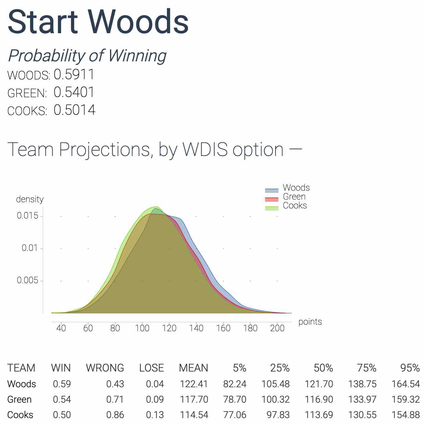
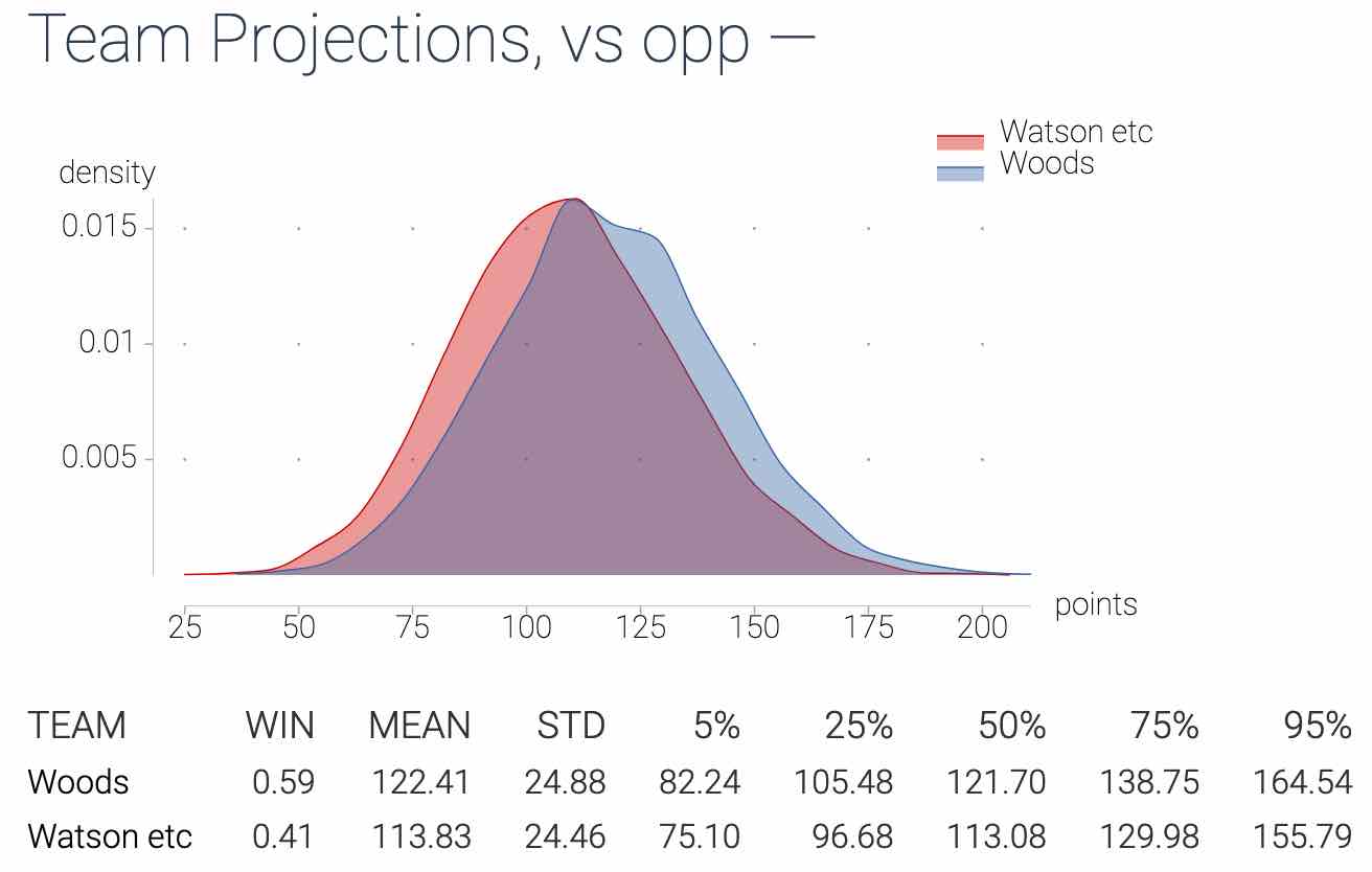
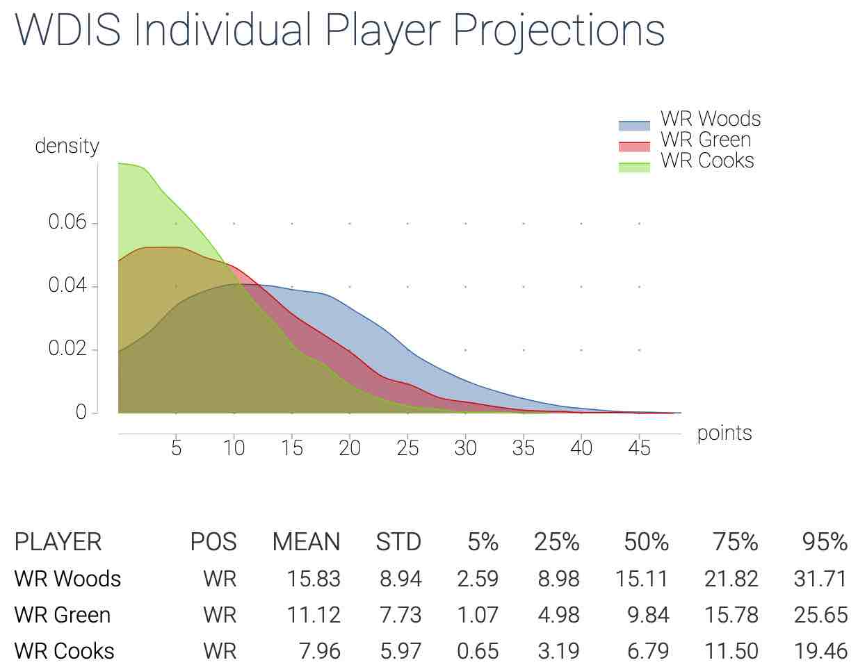
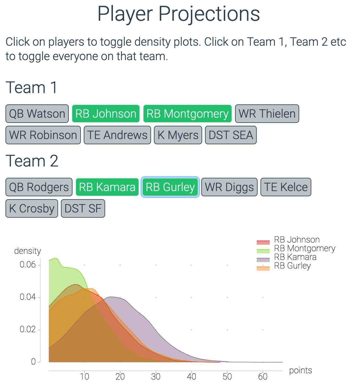
I built a web app that does this. I make the correlated simulations for every player for the upcoming week (updated automatically a few times a day to reflect e.g. injury news), then you can you put in your matchup and get back the projected scores and probability you win. You can also put in different guys, and it’ll run the scenarios and tell you who best maximizes your chances.
Other differences:
- more scoring systems (PPR, non PPR, half PPR, 6 point passing TDs, etc) — and more correlations since e.g. the correlation between a QB and his WR1 are different in PPR vs standard scoring
- more simulations. 10000 instead of 500. This helps detect every possible edge/squeeze out any noise.
- I’m working on getting it up and running for 2024, if you want get notified when it’s ready you can check it out here:
I’m also contemplating making the raw simulations (e.g. the sims and nsims data we’ve been working with above) more widely available, either as CSVs or via an API. Let me know if that’s something you’d be interested in.
Some screenshots from last year’s app:
Appendix - Fantasy points as distributions
Here’s a quick set of numbers –
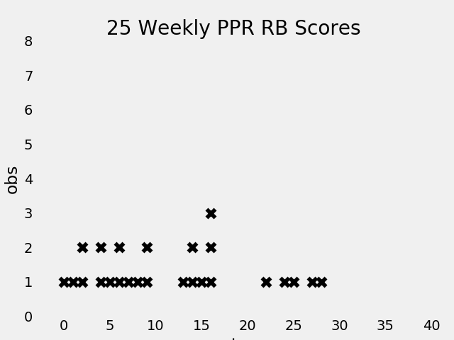
17… 24… 8… 4… 13… 12… 0… 15… 14… 13… 11… 7… 0… 8… 17… 23… 2… 15… 9… 4… 28… 5… 9… 5… 17…
These are 25 randomly selected weekly RB performances from 2019. The first is Todd Gurley’s 17 point performance in week 16, the second is Derrick Henry’s 24 point performance week 14, etc.
Ok. Now let’s arrange these from smallest (0) to largest (28), marking each with an x and stacking x‘s when a score shows up multiple times. Make sense? That gives us something like this:
Interesting, but why should we limit ourselves to just 25 games? Let’s see what it looks like when we plot ALL the RB’s over ALL their games:
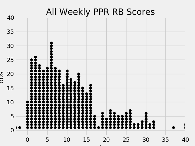
This is the first key to thinking probabilistically about fantasy football:
For any given week, when you start a player you’re picking out one of these little x’s at random.
Each x is equally likely to get picked. Each score, however, is not.
There are a lot more x’s between 0-10 points than there are between 20 and
30.
Distributions: Smoothed Out X’s
Now let’s switch from stacked x’s to curves, which are easier to deal with mathematically.
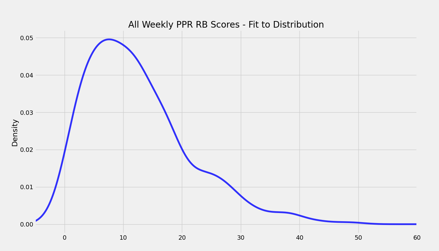
The curve above is called a distribution. For our purposes, they’re a way to smooth things out. We’re replacing the stacked x’s with a fuzzier, smoothed out curve. You can continue to imagine the area under these curves as filled up with little, stacked up x’s if you want.
The horizontal axis on this curve still represents fantasy points. The vertical axis is less intuitive, but it ensures the area under the curve equals 1. Don’t worry about it this if it’s confusing.
So you’re heading into the Monday night game up by 10 points. Your team is done and the guy you’re playing only has one RB left — how likely is it you come out with a win?
The answer — assuming your opponent is starting a random RB — is about 50/50. Half of the area under the distribution (half of the little x’s in Figure 2) is at 11 points or higher, half is below.
That’s if your opponent is starting a random running back. What if he’s starting Ezekiel Elliot?
Zeke is not some random RB. His score is, on average, higher than average, which means his distribution is further to the right. Something like the red one below.
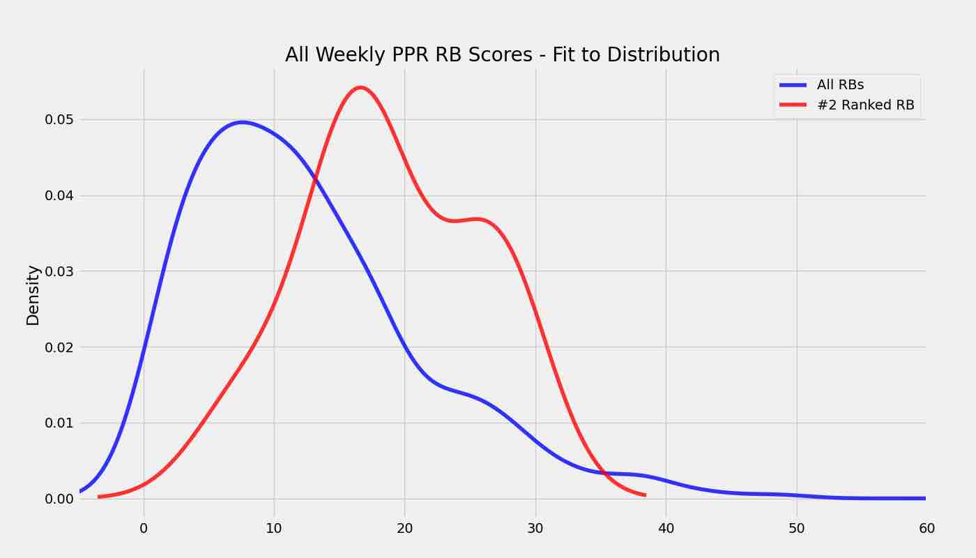
In that case, Zeke will score more than 10 points 90% of the time and things aren’t looking good for Monday night.
This is important: the shape of probability distribution changes for any given player and week.
A lot goes into these distributions: offensive line, quality of the defense, number of touches, whether the RB is in a committee, etc.
Your job as a fantasy player: assemble a lineup of guys with distributions far to the right.
This maximizes your chances of winning. Does this mean you’ll always win or start the right guy?
Of course not. Even above, a draw from a random RB’s distribution (the blue line) will be higher than a draw from Zeke’s about 20% of the time. But it will put you in the best position to maximize your odds.
The key is changing how you view player-performances. They’re not taken out of thin air, or something to be rationalized and fit into a narrative (I KNEW this [guy who performed poorly] was bad, never again!). That’s a recipe for frustration and chasing points.
Instead, view performances as random draws from some range of outcomes. This captures the randomness inherent in Fantasy Football, is a good model for what’s actually happening behind the scenes, and is a way to stay sane.